The average run goes for about 4.2 yards. The average NFL running back has an average YPC of about 3.5.
The three most common outcomes of a run every year for the past six years have been gains of 1, 2, or 3 yards (usually in the order of 2/3/1).
The 1-3-5 rule: Over a quarter of rushing attempts are over by 1 yard, about half of rushing attempts are over by 3 yards, and about ¾ of rushing attempts are over by 5 yards.
The 10 at 10 rule: any run that goes at least 10 yards is among the longest 10% of rushing attempts.
On the field, the ball is spotted “exactly”, but on the stat sheets, field position (and thus yardage) is rounded “up” towards the end zone to the nearest whole yard (except in some particular circumstances, such as when there is less than a yard to go for a first down, in which case the yardage is rounded down in order to leave 1 yard remaining for the first down instead of 0).
A rushing attempt can be thought of as taking a sample from a distribution of possible outcomes. Examining the distribution across runs for certain players and circumstances can tell us a lot about the nature of the possible outcomes for that players or circumstances. The distribution of all runs is significantly right-skewed (i.e. has a long right tail indicating that there are just a few runs that go for a very long yardage – the “bill gates” of runs).
A cumulative density plot shows the proportion of runs that make it to particular yardages.
There are three phases to a run: the yards that are blocked, the yards that are contested (where most runs are stopped), and the open field. The yards that are blocked are mostly “free” for the running back, who generally uses that time to rapidly approach the contested zone. In contrast, open field running has a special type of momentum: each step past the contested zone increases the expected yards remaining on the run. Running gets easier the further the running back goes.
20% of all RB runs in the NFL over the past six years are attributable to just ten players: Gore, McCoy, Lynch, CJ2K, Peterson, Forte, Foster, Steven Jackson, DeMarco Murray, and Morris.
Half of all active running backs over this 6-year period accumulated fewer than 60 total attempts. A quarter of all running backs since 2010 never made it past 15 total carries.
The run distributions reveal different running styles. We’ve identified six “archetypes”: High-volume Grinders, Home Run Hitters, Short-Yardage Bruisers, JAGS, Elite Pass-Catching backs, and Game-Breaking Talents.
Grinders include Gore, Morris, Ingram, MJD, Blount, and Lacy. Their value lies in maintaining a high usage rate without sacrificing efficiency in any part of the game.
Home Run Hitters include McCoy, Peterson, Forsett, Reggie Bush, and Christine Michael. Their value lies in tremendous open-field running that can kick-start a scoring drive.
Short-Yardage Bruisers include John Kuhn, Shonn Greene, Peyton Hillis, Daniel Thomas, and Law Firm. Their value lies in hitting the line hard and falling forward, reliably picking up at least a yard or two before going down.
JAGS have value mostly as depth. Most running backs on NFL rosters are JAGs or worse.
Elite Pass-Catching backs include Woodhead, Pierre Thomas, Sproles, Vereen, and Helu. Their value lies in their versatility, their ability to keep defenses honest as a dual threat, and their ability to exploit soft fronts.
Game-Breaking Talents include DeMarco Murray, Le’Veon Bell, LaDainian Tomlinson, and Jamaal Charles. They are good at all phases of the run even at a high volume.
Jamaal Charles looks like the greatest running back of the decade.
Run distributions are not known to be predictive, but Rawls, Karlos Williams, Jerick McKinnon, and David Johnson are looking very promising.
2008 sucked for the Pats.
Chapter 3: Finding Player Comparables through Distribution Matching
We can find the “closest” run distributions for different players using an algorithm to find the shortest distance between the curves. We used a few tricks and settled on “Nearest Neighbor Retrieval”.
Finding matches from the archetypes we explored last time allowed us to find other players who seem to belong to that archetype. CJ Spiller appeared to be a home run hitter, Jonathan Grimes a pass-catching back, and Fred Jackson looked suspiciously like a game-breaking talent.
The algorithm helped identify Matt Forte and Arian Foster (who are extremely closely matched) as an interesting case of elite pass-catchers who still run like Grinders (carrying a high volume when active and producing an output similar to Frank Gore).
“Backward matching” entailed the process of using older veterans to find younger players who are running in a similar way. Le’Veon Bell, Giovani Bernard looked a lot like FJax. Jerick McKinnon and David Johnson looked a lot like DeMarco Murray. Kendall Hunter looked like he maybe could have been a McCoy type runner.
“Forward matching” entailed the process of running the younger players through the algorithm to see which established players they most resemble. All of the rookie and sophomore running backs are described above, along with some notes.
The league-average yards per carry is 4.18, but we expect even perfectly average players to be higher than that sometimes and lower than that other times.
Smaller samples introduce more variance. In other words, increasing your sample size increases the precision of your sample mean.
Once we get to about 30-40 carries our so, a single freak long run or two is less likely to skew the whole Yards per Carry too much to the “big” side. A big enough room maybe couldn’t handle Bill Gates, but it could handle the odd millionaire without totally screwing with the average too much.
When we take the average of 10 random runs from the NFL, we get an average between 2.8 and 5.1 YPC only half the time.
Long runs are important for teams trying to grind out first downs on the ground. Home Run hitters were particularly good at gaining at least 10 yards when given 3 consecutive carries in our simulations. Short-yardage bruisers were particularly bad.
The majority of first downs in this 3-carry simulation came from a single run of 10+ yards (rather than a string of shorter runs). But the single distance that seemed to yield first downs most commonly was the 7 yard run. That’s the balance point between distance and probability (where 7 yards appears to be long enough to convert most of the time, but short enough to happen reasonably often).
The situation matters. Expected outcome of a run depends on the context (possibly through play calls by the offense and defense).
In general, when running is the more valuable strategy for the offense, the defense tries to take away that option, and running efficiency is reduced.
Rushing attempts on 1st and 2nd down go further than rushing attempts on 3rd and 4th downs.
Rushing attempts close to the line of gain tend to be shorter than rushing attempts further from the line of gain.
Down and distance are correlated for rushing attempts. More than half of all 3rd down runs by a running back take place within 2 yards of the first down, and more than half of 4th down attempts take place within 1 yard.
Within the 25, running the ball starts to become increasingly less efficient. Much of this difference is due to the goal-line cutoff (where it’s not possible to gain more yards past the goal line if you score a touchdown), but a half-yard of this decrease is attributable to other game factors (possibly defensive play calls and the compressed field).
There is also tentative evidence for a slight drop in running efficiency as the offense nears field goal range.
The complete model of down, distance, and field position indicated two major distince influences: 1) the goal line effect, and 2) a line of gain effect specifically on third downs (where running on a third and short is particularly hard). (Note: this “generalized additive model” essentially works by drawing flexible curves over the specified context features, then adding them together for any given rushing attempts).
Early in the game, the winning team is more likely to have better rushing attempts, on average. Late in the game, the losing team is more likely to have better rushing attempts. Being up 2 touchdowns in the 1st half or down 2 touchdowns in the 2nd half is worth about an extra half-yard.
The tendency for defenses to take away the run when running would be most valuable to the offense is exactly what we’d expect according to game theory: the ideal strategy for a defense is to guess the probabilities of different moves by the offense, and choose the best strategy against that guess.
As a consequence, football teams are incentivized to be unpredictable in their offensive play calls. Sometimes, the best offensive play is the suboptimal one, and that means running the ball sometimes even when passing might have a higher expected yardage.
Every run can be thought of as a draw from a probability distribution. That means that every distance gained has a probability of occurance.
We can estimate those probabilities using kernal density estimation.
Thinking in probabilities instead of distances solves the ‘long run problem’.
Given those individual run probabilities, we can calculate the probability of whole games.
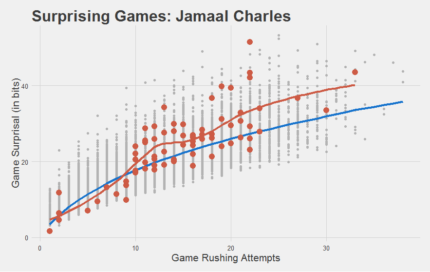
We can use information theory to convert those probabilities into interpretable values. Improbable games are more surprising, and more surprising games have higher “Surprisal”, a measure of information (in bits).
A 1-bit increase in Surprisal corresponds with a game that was half as probable (i.e. twice as improbable/surprising).
Game Surprisal is sensitive to both volume and efficiency. More efficient games are more surprising, but any particular high-carry game is also surprising (because there are more possible outcomes, spreading the probability around).
We can account for volume by simulating a league-average Game Surprisal for each number of carries in a game. This gives is “marginal game surprisal”, which we call Game Score.
Game Score is a pure, game-level efficiency satistic, measured in bits. A Game Score of 0 is average, given that many carries. A Game score of 1 is twice as improbable/surprising as an average game. A Game Score of 2 is 4 times as improbable as an average game (i.e. twice as far from average as a Game Score of 1).
Game Score passes the eye test: it thinks Jamaal Charles, LeSean McCoy, Adrian Peterson, and DeMarco Murray are good, and it thinks Trent Richardson is godawful bad.
Game Score is significantly more stable from year to year than yards per carry.