- The Signal and the Noise
- Foot Race: Running Head to Head
- How the Sample Got Its Size
- Foot Race revisited: Unleash the Kraken
- Simulating a Series
- CHAPTER SUMMARY
The Signal and the Noise
Bernie, can I tell you one of my pet peeves?
 “Fruit that never seems to get ripe no matter how long you wait?”
No. I… wait what?
“Fuckin’ pears, man.”
…OK maybe that too, but I mean one of my biggest football-related pet peeves. You know what? Just look at this quote:
“T.J. Yeldon has not established himself thus far during his rookie campaign, but he did score for the first time last week via reception. The Alabama product has averaged 3.0 YPC or less in three of his four games this year”
“Well to begin with, that’s not even correct. His first score came in week 5, when this was written, so that should say ‘three of his five games this year.’ But even if this particular fantasy site had even bothered editing this for typos, these ‘stats’ are almost totally meaningless.”
Right? Like, let’s look at the game log here. The three games in question are week 2 vs MIA (25 carries, 2.8 YPC), Week 3 @ NE (11 carries, 3.0 YPC), and Week 5 @ TB (11 carries, 2.9YPC). Even if they hadn’t fucked up their own stat, and even if the “3.0 yards per carry or less” wasn’t totally arbitrary, and even if it wasn’t trivially true that “about half your games will be below average and about half your games will be above average” (note: his next game, he stomped all the fuck over Buffalo for 115 yards and a touchdown), this would still be a shit stat.
Here’s the thing: what we’ve got here is failure to communicate appreciate the difference between the signal and the noise.
“In statistics, the ‘signal’ is the systematic relationship of interest. A link between a predictor variable (like “player”) and an outcome measure (like “yards per carry”) that is the ‘true nature of things’ that you hope to uncover. If Trent Richardson really, truly sucks, then no matter how many times we look, we should find that he sucks more often then not (assuming we know what we’re doing when we take a look). The “noise” is everything else that we didn’t (or can’t) account for. Sometimes, if we happen to look at just the right time, Trent Richardson may manage a respectable carry. Does that mean that he’s better than we thought he was? That he’s good all of a sudden? Or was it just random chance?”
This is critical in the evaluation of rookies. Even if you ignore their potential for development (which, as we explore in a quick hit, doesn’t seem to actually happen much), how do you know whether they are good or bad in the first place? Let’s say some new rookie takes ten carries for an average of 3 yards per carry. Is that ‘signal’? Telling us that the rookie is below average? Or could that just be ‘noise’? The type of game that we completely expect to see now and then even from an established vet like Marshawn Lynch? What if it was 20 carries instead? Is that enough? 30? 50? What if they took 100 carries for 5.0 yards per carry average? Can that happen by random chance, from a completely average running back? Or is that the signal that he’s probably pretty good?
“This was what we're illustrating with the Yeldon quote above. The problem here is that the writer just assumed that the low YPC for those games was ‘signal’ instead of noise, and didn’t bother to ask how probably it was that this was something we could have seen by chance.”
I can’t really blame them, to be honest. It’s just not too common to address random chance in NFL writing in any sort of systematic way.
Well, you know what? That ends today. We are about to analyze the shit out of the role of chance in the run game.
Foot Race: Running Head to Head
Let’s start with a simple wager. We’ll pit two players against each other: Trent Richardson versus Beast Mode. We’ll pick one rushing attempt at random from each player. We look at instances where they were handed the ball in a real game, and see who takes it further. You can have Lynch. If Beast Mode has the longer run, you win. If he doesn’t, we win.
What kind of odds will you give us? 1.5 to 1? 2 to 1? 3 to 1? 5 to 1? In essence, how likely do you think it is that Lynch has the longer run?
“It’s actually a very simple matter to simulate this head-to-head competition. I have every Richardson run from his entire career, and every Lynch run from 2010 (the point at which he was clearly awesome) through his recent retirement. I can just take one of each, at random, and see who had the longer run. In fact, in the time it took you to read this, I’ve already simulated the competition 10,000 times. BAM! I’ll put the results below. But I want you to think of a number in your head before you do: what proportion of the time does Lynch run further than Trent Richardson on any given carry?”
Let that sink in for a second. I assure you that we did this correctly, that Trent is just as bad as you think he is, and that Beast Mode is just as good as you think he is.
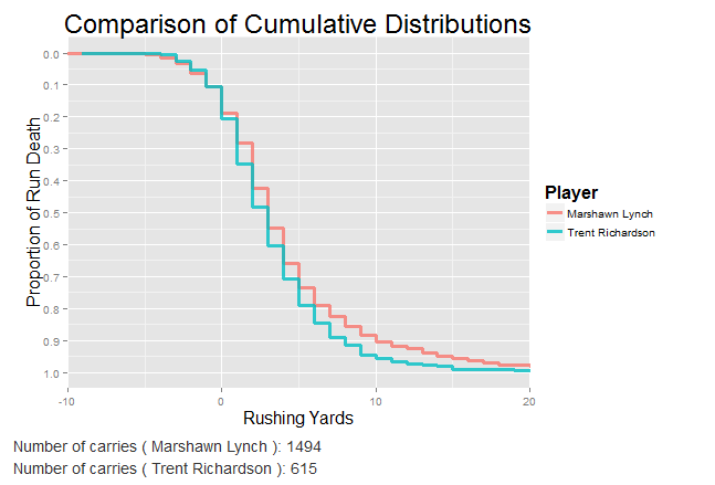
We have quadruple-checked this simulation, and have posted the code online so that everybody can see for themselves too. You can even check yourself with the app. So what’s going on here?
“Some of you may have already landed on the problem: our sample size was too small. They just took a single run. That’s not really ‘enough’ to really let Lynch’s skill to come through.”
But that’s exactly the point. Everybody already intuitively knows that those Trent wins were just noise, not evidence that Trent was awesomer than Marshawn Fucking Lynch. We tried to draw a conclusion too fast. But now the question is ‘how many carries is enough’?
Tell you what, let’s do the bet over. This time, we’ll give them each 11 carries. That’s the same number of carries that Yeldon had in those two games that so concerned the fantasy writers we quoted. 11 carries is a good number, right? If Beast Mode already had an advantage when we gave them each 1 carry, giving them an order of magnitude more carries should let Lynch win almost every time, right? Would you give me 3 to 1 odds? 5 to 1? 10 to 1?
“I’ll just run my simulation again, taking 11 random runs from each of them, then repeating the process 10,000 times, and…”
Crazy right? I promise you we haven’t fucked this up. Those are the real numbers.
Just to assure you that is possible to tell from the numbers that Lynch is probably better than Trent, we calculated the approximate number of carries that you would need to give each of them in order for Beast Mode to win 95% of the time. Turns out to be 130 carries.
“My favorite part of that little factoid – you know how many carries Trent had when the Colts swapped a first round pick for him?"
How the Sample Got Its Size
So what the hell is going on here? Let’s take a step back for a moment. Look at the big picture. Say we just take 10 carries at random from the past 6 years (across all players). What kind of yards per carry averages do we expect to see? Remember, the league-average yardage is 4.18, but we’re only averaging together 10 runs at a time, so we probably won’t hit 4.18 exactly whenever we do this with only 10 carries – we expect to be higher sometimes (maybe they bust out a long run) and lower other times (maybe they got stuffed a few extra times). The small sample introduces some random variance.
We do it once: 4.7 YPC.
We do it again: 6.5
Again: 2.8
More times: 4.7, 4.2, 5.2, 11.7, 3.0, 3.1, 5.5
“We do it 10,000 times. We get this distribution.”
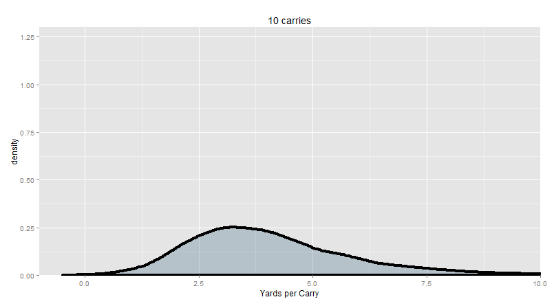
“The ‘center mass’ of this distribution is about 2 to 5 YPC. More precisely, when we take the average of 10 random runs from the NFL, about half the time, we get an average between 2.8 and 5.1 YPC. And anything between 1.3 and 9.2 YPC is not too strange – 1 in 20 of our samples were even more extreme than that. A single 90-yard run would change the YPC quite a bit!”
In other words, a league-average running back will produce a yards per carry below 3 or above 5 more than half the time when your sample size is only 10 carries. It doesn’t necessarily mean that the running back is below average or above average as an individual. It just means that your data is completely consistent with the sort of random variance we expect from a perfectly average player.
“Now let’s take the other extreme. Let’s say you have a league-average running back that you can somehow give a billion carries to. Actually, scratch that – let’s make it a billion billion carries. Let's just assume that this particular player doesn't get tired, and doesn't age, so his yadrs per carry is, on average, the same for all billion billion carries. I don’t even need to simulate this to tell you what his yards per carry is going to be. It’s going to be pretty much exactly 4.18. The league average. Just like we all know that 1 is too small of a sample, we all know that a billion billion is probably big enough. So big, we’ll get a really precise measure of the ‘true’ yards per carry – exact to some large number of decimal places that we don’t really care about. The key is how you get from 1, to 10, to a billion billion. What actually happens when you increase the sample size? Your estimated yards per carry should get more and more precise, right? In other words, this distribution of sample means (like the one we showed you above) should shrink when your sample size is larger, because any given sample mean is closer to the ‘truth’.”
Here’s 25 carries in each trial (across 10,000 trials), which is about the size of a single game for a high-volume feature back:
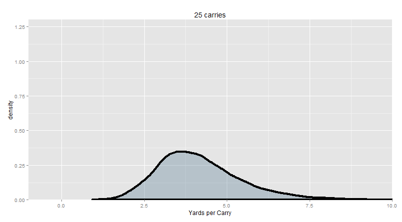
95% of our trial (or “sample”) means are between 2.16 and 7.16 yards per carry.
And here’s 100 carries in each trial, about equal to a month’s worth of carries for a high-volume feature back:
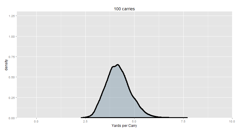
95% of our trial means are between 3.07 and 5.03 yards per carry.
And here’s 350 carries in each trial, about a season’s worth of carries for a high-volume feature back:
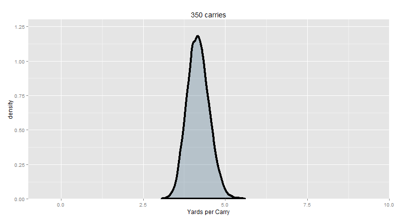
95% of our trial means are between 3.56 and 4.86 yards per carry.
“I think you see where this is going. The bigger your sample, the more precise your estimates are. The closer it gets to the “true” average (in this case, known to be about 4.18, since we’re looking at the typical run). So behold: this is how you go from ‘too small’ to ‘enough’ of a sample:”
God, isn’t that beautiful? Let this sink in for a while. This is, no joke, quite possibly the most important concept in all of statistics.
Of course, you know what else is beautiful? Telling people that they are wrong on the internet. To that end, we have put some key information from this plot into argument-table format for you.
When you see somebody throwing around yards per carry with small sample sizes, say: “Well actually, if your sample size is around [N], then any yards per carry average between [Blah and Blah] could easily be explained by the random variance of a perfectly average running back.”
| [N] | [Blah and Blah] |
|---|---|
| 10 | 2.80-5.10 |
| 15 | 3.06-5.00 |
| 20 | 3.25-4.90 |
| 25 | 3.28-4.88 |
| 30 | 3.37-4.87 |
| 40 | 3.48-4.78 |
| 50 | 3.54-4.70 |
| 75 | 3.65-4.62 |
| 100 | 3.74-4.57 |
| 150 | 3.81-4.49 |
| 200 | 3.87-4.46 |
| 250 | 3.90-4.42 |
| 300 | 3.92-4.41 |
| 350 | 3.95-4.39 |
| 400 | 3.96-4.38 |
“For the curious, these numbers are the “50% confidence intervals” for the distributions in the gif. A very informative and criminally under-utilized indicator. Essentially, a perfectly average running back is twice as likely to produce a yards per carry inside the listed range than below the range, but also at the same time twice as likely to produce a yards per carry inside the range than above the range. Overall, the “middle half” of the YPC produced by a perfectly average running back will be inside the range.”
I want to unpack this just a little bit more. Let’s say we have an 11-carry game from T.J. Yeldon, and he goes for 3.0 yards per carry. Because he’s a rookie and we don’t really know how good he is yet, we want to compare him to the average, essentially answering the question of “do we think he’s below average yet?” Clearly, we can’t just conjure a larger sample from T.J. Yeldon, or have him replay the same 11 carries 10,000 more times. But we do know what average looks like (see: chapter 1. In fact, we can simulate the answer to the question of “what does 11 carries from a league-average running back look like” to produce basically as much data as we want. So instead of asking “is T. J. Yeldon average or not”, we flip the question, and ask “is T.J. Yeldon’s output something that a league-average running back could have produced by random chance?”. In statistics, we usually set the cutoff at 95%. If 95% of the league-average samples of 11 runs produce a yards per carry are less extreme than T.J. Yeldon’s single sample, then we would decide that we have sufficient evidence to conclude that he is different from the league average. Above, we show the 50% cutoffs instead. If T.J. Yeldon’s 11 runs produce a YPC below the listed range, it doesn’t necessarily mean that we can write him off. But if his YPC is inside the listed range, we really have no grounds whatsoever from which to conclude that his YPC is any different from the league average.
“But there’s a broader point here too that extends well beyond individual players. That gif is so important because it illustrates how exactly the size of your sample influences the precision of your estimate for what the mean is (and yards per carry is just a sample mean). In fact, the concept that we’ve demonstrated here already has a name: the Central Limit Theorem.”
The Central Limit Theorem can be thought of as having two parts, and both are completely apparent in the gif. Part 1: Increasing your sample size increases the precision of any particular sample mean (on average). Or rather, how precisely your sample mean reflects the ‘true’ mean. When our sample size is about 10, like it was for T.J. Yeldon, even a league-average running back could give us a yards per carry anywhere inside of a HUUUUUGE range.
But at 350 carries, a league-average running back should have a yards per carry that’s pretty close to reflecting the ‘true value’.
Totally sensible, right?
“It turns out it’s actually very easy to calculate how “far” your sample _probably_ is from the mean with just a few simple assumptions (we actually violate some of these assumptions, particularly the assumption that our data points are all indepedentant from one another, but we can still use the CLT to ballpark how precise our estimates might be). Just take the standard deviation of the run distribution (i.e. where the samples are coming form) and divide by the square root of your sample size. Part 1 of the CLT is pretty easy to prove if we start from here: as the sample size gets bigger, the standard deviation of the sample means gets smaller, because you’re dividing by a bigger and bigger number (so there is less spread).”
Alright Bernie, let’s try to avoid the hardcore math, please? In any case, Part 2: once your sample size is big enough, the sample means will be pretty symmetrically distributed, regardless of how fucked up the original distribution looked.
You remember the original distribution (that we’re taking samples from):
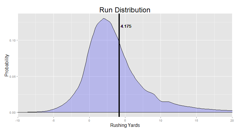
Not symmetrical. Big old tail on the right. But if we take 10,000 sample means, each with a sample size of 350, we get this:
The tail on the right went away. You don’t even need to worry about it. This is critical, because it means that we don’t need to worry about being prone to systematically overestimating or underestimating a player because of a weirdly skewed initial distribution (i.e. we don’t need to be too worried about the Bill Gates effect we talked about previously). If our sample size is big enough, the sample mean has about an equal chance to be “off” in either direction, and would be “off”, on average, by about the same amount.
“For part 2, ‘big enough’ turns out to be about a sample size of about 30. “Infinity” is ideal, but more or less 30 is enough. So statisticians have a joke that they like to tell each other a lot: ‘As you know from teaching introductory statistics, 30 is infinity.’ Get it? Because a sample size of 30 is basically just as good as infinity if you want to use part 2 of the central limit theorem? Trust me, if you ever meet a statistician, work this joke in somewhere. It kills.”
Foot Race revisited: Unleash the Kraken
So let’s say that instead of comparing T.J. Yeldon to “the league average,” you instead want to compare one running back to another, like we did above comparing Lynch to Richardson. Well now, you have two potential sources of variance. There’s randomness in how precisely your sample reflects the ‘true’ Beast Mode, AND there’s randomness in how precisely your sample reflects the ‘true’ Trent Richardson. Small samples are less precise, and big samples are more precise. But with so much random chance involved, is it any wonder that Beast Mode lost to TRich in a 10-carry contest about a third of the time? There’s too much noise!
“So let’s improve things, shall we? We started with 10 runs each. That looks like this:”
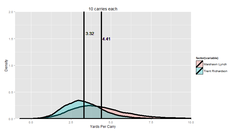
The colored curves are the distribution of the their 10-carry competition runs (in yards per carry). The bars are the average of all the averages (Lynch on the right, TRich on the left).
“Now let me slowly dial up the sample size for you.”
By the time we get to pretty much the max possible number of carries in a season (only five players have ever surpassed 400 carries in a regular season, and each one of them only did it once), Marshawn Lynch wins 99.9% of the time. You can just barely see the narrow sliver of overlap where it’s even possible for TRich to win. Essentially, TRich needs to get lucky with a 1 in 100 great season (maybe a couple of 80-yard runs go his way, just by random chance) AND at the SAME TIME, Beast Mode needs to have god-awful luck with a 1 in 100 BAD season.
“Now, so far, we’ve been discussing the role of randomness in how it might influence our player evaluations. Luck plays a big role in output, and it’s important to factor it in. But if you think about it, there is one very real, very tangible way in which understanding random chance has a profound influence on football strategy during the game itself.”
You have the ball at your own 20. It’s a first and ten. Lynch is healthy. If you gave it to Beast Mode three times… what are your chances of getting a first down?
Simulating a Series
You can probably intuit how we might approach this question, given the simulations we’ve run above. Lynch doesn’t get 3 consecutive carries in a series enough to really say with confidence what his probability of a first down will be, but we know what his run distribution looks like, so we can simulate giving him 3 carries by sampling 3 random carries from his real, actual game history. Essentially, we can just pick three random Marshawn Lynch runs out of a hat, pretend that they were consecutive, and see whether he gains a first down with them. This approach has limitation, of course, but can still be enlightening for our purposes of examining the impact of random chance.
“As usual, we repeat the process 10,000 times. When you do that, it turns out that when you simulate handing the ball to Lynch three times in a row, he’ll gain a first down about 58.5% of the time. That’s lower than the 66% rate that teams usually gain first downs with, but perhaps not by as large a margin as I would have expected for a scenario where you don’t move the ball through the air at all. But the key point here is that Lynch’s average yards per carry over this time span – 4.4 – seems like it should be plenty to gain 1st downs reliably. Three of those is over 13 yards. But because of the randomness involved, he only makes the first 58.5% of the time.”
But we’re just getting warmed up here. We can also keep track of what Lynch needed to do in order to gain a first down. For example, he could simply just break out a ten-yard run (assuming he hasn’t lost yardage) and gain the first down all at once. But theoretically, he could also simply string together a couple 3-5 yard runs and grind out the required yardage. This is essentially a question of comparing two relatively small probabilities: long runs don’t happen very often, but you only need one of them, while short runs may happen more frequently, but you need to string together three in a row, which may not be particularly likely. So which is it? Is Lynch mostly gaining those first downs from big runs? Or is he grinding them out from a series of smaller runs?
“Looking at the longest run of the three carries is one way to assess this. Lynch only makes it 10 yards (or more) with a carry about 10% of the time. But 52% of his first downs came from a run at least 10 yards long. This seems to indicate that the low-probability “home runs” are particularly important for a running back to gain a first down on his own (starting from a first and ten).”
Another way of looking at it is this: if your longest run is X yards, what are your chances of still gaining a first down? Here’s the splits for this Marshawn Lynch 3-carry simulation:
| Longest Run | First Down |
|---|---|
| 5 | 35.6% |
| 6 | 56.4% |
| 7 | 70.6% |
| 8 | 84.2% |
| 9 | 88.2% |
This makes sense: if your longest run is 6 yards, then your other 2 carries have to go at least 4 yards total. If your longest run is 8 yards, then your other 2 carries have to go only 2 yards total. A long run makes it a lot easier to gain a first! But the actual impact is pretty striking: only 36.5% of first downs come from series where Lynch has a long run of 8 yards or less.
“These data seem to indicate that grinding out first downs on the ground is pretty hard – most first downs from Marshawn Lynch came from his ability to break out a long one. It signifies that those long runs may be significantly more valuable for a high-volume back than the ability to grind out short yardages reliably. You know who’s good at long runs? Home Run Hitters. Lynch (no slouch at the long runs himself) gained the first down about 58.5% of the time. LeSean McCoy, the classic home-run hitter, gained the first down about 60% of the time in these simulations. And that’s despite the fact that McCoy is more likely than Lynch to lose yardage on a run. Frank Gore is a better short yardage runner than McCoy, but it turns out that he only makes the first down in this simulation about 55% of the time in a 3-carry simulation. John Kuhn, our examples of a classic short-yardage specialist (but terrible open-field runner) only makes the first down about 43% of the time.”
This is a pretty clear pattern. If you want to get a first down on the ground, starting from a first and ten, you want the home run hitter. The Bruiser has his place, of course: remember, if you get yourself to a 3rd and 1, Kuhn is much more likely to get you that last yard than McCoy is. I speculate that if we incorporated the passing game here (where 6-10 yard passes are common), Bruisers would show their value more. But to get that first big chunk on the ground exclusively, you want to gamble on the boom-bust guy.
“This isn’t a general rule, of course. Like we told you right at the beginning of Chapter 1, the “right” call is nearly always situation-dependent (rather than statistically contingent). What if you have Brady as your quarterback and trust your ability to pass for 5-6 yards pretty reliably? What if the defense is showing you a particular look? And I’d also mention that you don’t need to gamble on the boom-bust guy if you have a game-breaking talent on your roster. Jamaal Charles makes the first down 67.5% of the time, and he’s got no problem running for short yardages too.”
Alright, we’re not doing the Jamaal Charles love-fest again. But you have a great point here: the situation matters. And if I’m honest, we probably don’t want to just assume that running on a 1st and 10 is identical to running on a 3rd and short. The type of defensive fronts and offensive play calls from the two are really, really different.
Well, we can handle that too. Let’s say our simulation starts with a first and 10. We can sample a random run only from actual 1st and 10 situations. That way, the yardage gained should be representative of what you might actually expect from a 1st and 10. Let’s say they go 4 yards. Now, we can sample random run only from actual 2nd and 6 situations etc. We’re really spreading ourselves thin here, so we wouldn’t have enough data from any one single player. But we should have enough, just about, if we look across the league as a whole.
“This takes significantly more computer power, but it was a fun little exercise. In the end, using this situation-adjusted sampling method, our league-average runner gains the first down about 58.5% of the time, but we still see a huge dependence on longer runs. When our longest run is 4 yards, we only gain the first down 12% of the time. When it’s 6 yards, we gain the first yard 62% of the time. When it’s 8 yards, we gain the first down 83% of the time.”
It’s nice to have the exact numbers, but again, this shouldn’t be too surprising. Long runs are harder to get, but when you get them, you’re more likely to get a first down. But there’s one last logical question to ask, then. Where’s the balance point? What’s the ‘sweet spot’ in yardage gained that strikes a balance between having a reasonable chance of occurring, but still making a first down very likely? Essentially, when we look at all of our successful conversion, what’s the run that pops up the most?
“I can answer that with a picture. Here’s a plot of where the first downs come from when you simulate running 3 times. It starts at 4 yards, because it’s not possible to get 10 yards in 3 attempts without at least one of those runs being recorded as 4 yards. Then it continues: how many 1st downs come from a series where you break out a 5 yard run, how many come from a series where you break out a 6 yard run etc all the way to 20 yards. The sweet spot is going to be the maximum of the curve.”
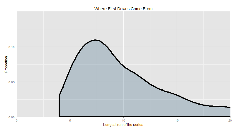
In short, the sweet spot is about 7 yards. Given the typical types of running output that happen at the different down and distances, if you want to get a first down exclusively on the ground, look for the 7 yard run.
CHAPTER SUMMARY
- The league-average yards per carry is 4.18, but we expect even perfectly average players to be higher than that sometimes and lower than that other times.
- Smaller samples introduce more variance. In other words, increasing your sample size increases the precision of your sample mean.
- Once we get to about 30-40 carries our so, a single freak long run or two is less likely to skew the whole Yards per Carry too much to the “big” side. A big enough room maybe couldn’t handle Bill Gates, but it could handle the odd millionaire without totally screwing with the average too much.
- When we take the average of 10 random runs from the NFL, we get an average between 2.8 and 5.1 YPC only half the time.
- Long runs are important for teams trying to grind out first downs on the ground. Home Run hitters were particularly good at gaining at least 10 yards when given 3 consecutive carries in our simulations. Short-yardage bruisers were particularly bad.
- The majority of first downs in this 3-carry simulation came from a single run of 10+ yards (rather than a string of shorter runs). But the single distance that seemed to yield first downs most commonly was the 7 yard run. That’s the balance point between distance and probability (where 7 yards appears to be long enough to convert most of the time, but short enough to happen reasonably often).